Why should current-day AI researchers look into biology and the brain? Artificial neural networks (ANNs) make up a significant portion of machine learning and deep learning, ranging from simple, early networks consisting of only a handful of neurons, to more recent networks with hundreds of billions of parameters (e.g., GPT-3). Despite the clear success of ANNs, there is clearly much that we can still learn from biological systems, which have evolved an amazing variety of solutions to solve the same challenges that AI engineers face.
At their inception, ANNs were inspired by biology and the human brain. The first ANN, called Logical Threshold Unit, was even conceived as a simple model of the “brain net”. In 1958, the psychologist Frank Rosenblatt proposed the perceptron, an early algorithm for supervised learning and a simplified model of biological neurons. Despite setbacks such as that triggered by the controversial book Perceptrons by Minsky and Papert (1968), the perceptron has remained surprisingly stable since then and underpins the incredible advances of modern AI.
Although they shared a common starting point, however, the AI and biological research communities diverged, and developments in the understanding of neural networks became community specific. While some ANNs take more direct inspiration from biology than others, e.g. spiking neural networks, essential tools developed by the AI community for ANNs, such as learning via error backpropagation, do not appear to have direct analogues in biological neural networks.
The success of modern AI, particularly deep learning, is an incredible testament to the usefulness of the tools developed over the past 60 years of neural network research. However, given that biology does things differently, we must ask whether there remain things that we can learn from nature to extend the capabilities of AI further still.
A pattern often seen in the literature is that a by-product of building ANNs that are more biologically plausible is an improvement in efficiency (memory, execution time, hyperparameter tuning, etc.) while reaching near-SoTA-level performance, e.g. Crafton et al., 2019; Lagani et al., 2021. This is observed across several datasets, metrics, network architectures and tasks, which hints at the overarching benefit of developing biologically inspired ANNs.
To keep the scope of our literature review manageable, we have identified three main topics (however this is by no means exhaustive):
- alternatives to backpropagation with gradient descent
- alternatives to the network architecture
- alternatives to activation functions and attention mechanisms
We have condensed our literature search into the figure shown in Figure 1.
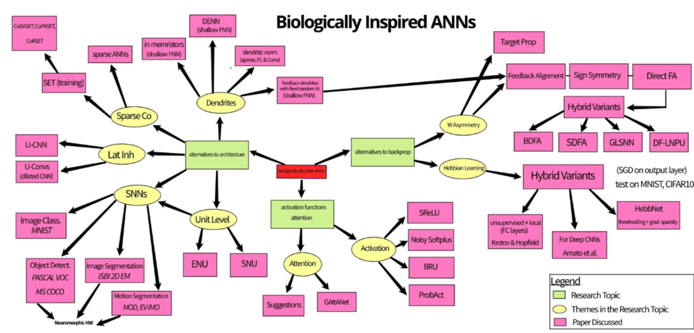
Figure 1: Mind map of three research themes on biological plausibility in ANNs
Focus: Alternatives to Backpropagation
Since the popularisation of backpropagation (1980s), researchers have made several attempts to find learning alternatives, often looking to biology for inspiration.
Before going into these biologically inspired alternatives, let’s briefly mention the two main reasons why backpropagation is thought to be implausible in biological neural networks:
- the weight transport problem: we need to “transport” the weights of the forward pass to the backward pass for the weight update computations, in which we use the transpose of the feedforward weight matrices W. There is no known mechanism in biological neural networks that would allow such storage and transfer of weights from the forward to a backward feedback pass.
- the update-locking problem: in backpropagation, weight updates only occur after a full feedforward pass. The timing of feedback signals in the brain differs from those in backpropagation-trained ANNs, and they vary depending on the biological neural network, e.g. see pyramidal neurons and their apical dendrite. There is no universal and precise definition of what feedback for learning looks like in the entire brain.
1) Hebbian Learning
Hebbian learning is directly inspired by the early biological experiments on human learning and neural plasticity in the brain. Nowadays, it has many variants with differing levels of acceptance in the neuroscientific community, but the first formulation of this rule dates to the 1950s with “Hebb’s Rule” (Hebb, 1949). It is an unsupervised learning rule, considered the foundational or simplest account of biological learning.
A limitation of naïve implementations of Hebb’s Rule is the problem of boundless growth. Given this rule, weights are indefinitely and exponentially increasing throughout training. Strengthening the connection between the neurons increases the firing rate, which in turn strengthens the connection, causing a runaway positive feedback loop.
One recent paper based on this simple formulation of Hebb’s Rule is Gupta et al.’s work (2021), called “HebbNet“, which attempts to address this boundless growth problem.
HebbNet is a shallow fully-connected neural network with one hidden layer of 2000 units. The output layer’s weights are updated using gradient descent while the hidden layer training is achieved via one of three Hebbian-like learning rules: the simplest version (Hebb’s Rule); Hebb’s rule with thresholding; or Hebb’s Rule with thresholding and gradient sparsity (not all weight matrix elements are updated at each backward pass).
There are also other ways of addressing the issue of boundless growth in Hebb’s Rule, such as Oja’s Rule (Oja, 1982) and spike-timing-dependent plasticity (Makram et al., 1997; mostly used in spiking neural networks). Oja’s Rule is a mathematical formulation that addresses the issue of boundless growth by introducing a “forgetting” term. In Figure 3, we include results when replacing Hebb’s Rule with Oja’s Rule in the setup from the HebbNet paper.
We attempted to reproduce the results from the HebbNet paper, and to compare with Oja’s rule. Figure 3 shows test accuracies on MNIST and CIFAR-10. Note that we used the same hyperparameter configuration as in the paper, except for the learning rate ( to avoid floating point overflows due to runaway weight growth) and the gradient sparsity (we fixed it to p=0.3, i.e., only 30% of the weight matrix is updated at each backward pass, whereas the paper mentions using an optimal value).

(HL = Hebbian Learning; T: Thresholding; GS: Gradient Sparsity)
As expected, “Vanilla” (that is, the original formulation of) HL performs poorly in the MNIST classification, regardless of the rule used. Surprisingly, for the CIFAR-10 classification, the three different versions of the Hebbian-like learning rule all perform similarly. We note that our results are considerably lower than those reported in the paper. Moreover, Oja’s Rule generally outperformed Hebb’s Rule in our experiments.
In the HebbNet paper, Hebbian learning and backpropagation with gradient descent are used separately for the training of different layers: the former for the hidden layer, the latter for the output layer. This makes it difficult to advocate for the use of Hebbian Learning during supervised training since, by contrast, backpropagation is appropriate for the training of all layers in the network. The increased complexity of having two learning methods for one network seems disadvantageous.
Given this, we have investigated ways in which shallow, fully-connected neural networks may be trained with the same learning algorithm/rule for all layers. To begin with, to train the same network with one hidden layer, we modified the conventional gradients’ definition in backpropagation by adding the unsupervised Hebbian Learning rule. That is, the gradients become the following simple “sum rule”:
gradient = gradient from backpropagation + β * Hebbian learning rule (either Hebb’s or Oja’s Rule) where β is a scaling factor (e.g. β=10e-2)

We trained the network with either Hebb’s or Oja’s Rule in simple Gradient Descent + Hebbian learning updates.
Figure 4 shows the test accuracy with respect to the Hebbian learning scaling factor β, where the rule used is Hebb’s Rule.
For MNIST, Oja’s Rule led to lower test accuracies (around 30%); for CIFAR-10, results with Oja’s Rule are like the results with Hebb’s Rule reported in Figure 4.
In both classification tasks, the smaller the contribution of Hebbian learning, the greater the test accuracy. With the smaller scaling factors, the test accuracy obtained with this sum rule matched the performance achieved with backpropagation on both datasets. These results suggest that adding a Hebbian learning component in this way does not confer any benefit over backpropagation.
Attempts to come up with single learning rules have also been documented in the literature. In 2019, Melchior and Wiskott proposed “Hebbian Descent“, a biologically inspired learning rule that can be repurposed for both supervised and unsupervised learning.
We have specifically focused on the supervised learning scenario, where we investigated the classification performance of shallow fully-connected networks (same as HebbNet) on MNIST and CIFAR-10.
Departing from this paper, we also examined replacing the centred input factor in the update rule (supervised learning version: Equation (6), see p.6) with Oja’s Rule. Figure 5 shows test accuracies on MNIST and CIFAR-10, where BP refers to backpropagation. There are three training versions: Full (both hidden and output layer weights are updated), Partial 1 (hidden layer weights are frozen), Partial 2 (output layer weights are frozen).

Backpropagation outperformed Hebbian-Descent on both datasets, although Hebbian-Descent (Hebb’s) performed very similarly on MNIST. Further, on MNIST, there seems to be little advantage to performing Hebbian-Descent on all layers as opposed to only some (the “partial” results, which is not observed on CIFAR-10: this is likely due to MNIST being relatively easier than CIFAR-10, where frozen weights do not hinder classification. On both datasets, the modified rule with Oja’s Rule fell behind.
In summary, the simpler variants of Hebbian Learning (Hebb’s Rule, Oja’s Rule) do not appear to match the accuracy of networks trained with conventional backpropagation. The most promising results (near-backpropagation level) were obtained when they were used in combination with gradient descent (e.g. Hebbian-Descent from Melchior & Wiskott, 2019). We suspect that more recent variants of Hebbian learning may perform better (e.g. spike-timing-dependent plasticity; there are multiple other learning rules which originated from Hebb’s rule). In all cases, simple Hebbian learning variants do not seem to be the whole story; they may work better as part of more complex learning rules and/or for training networks with specific configurations (such as the STDP rule being used in spiking neural networks).
2) Feedback Alignment Methods
A group of learning algorithms, called Feedback Alignment (FA) methods, were introduced in the community in 2016, and deal with the weight transport problem. The initial Feedback Alignment algorithm was documented by Lillicrap et al. in 2016 and later the same year, Nøkland proposed an extension, called “Direct Feedback Alignment” (DFA).
The idea is simple. Both algorithms make use of fixed random matrices as their feedback weight matrices. Essentially, the transpose of the feedforward weight matrix W (WT) becomes B, where B is a fixed random matrix defined before training. This way, we do not need to store and use the transpose of the feedforward weights. DFA goes a step further than FA by updating the earlier hidden layers of the network using the gradient from the output layer instead of the gradients from the higher-level hidden layers. Refer to the figure below, taken from Nøkland (2016), to visualise these algorithms (BP: backpropagation).

Below, we report classification results for networks trained using either FA (Figure 7) or DFA (Figure 8) for 300 epochs; the networks have either one hidden layer (2000 units; ReLU) or two hidden layers (800 units each; ReLU/Tanh layers; with biases)
We tried four ways of defining the feedback matrices B:
- fixed random: as in the 2016 papers on FA and DFA
- fixed random (sign): like the fixed random matrices but here the sign is congruent with the feedforward matrices W at each pass (similar to another algorithm called “sign symmetry”)
- fixed binary: B is a fixed matrix of randomly chosen -1s and 1s
- binary (sign): B is a matrix of 1s, and the sign is congruent with the feedforward matrices W at each pass.


Results from FA and DFA are less clear-cut than the Hebbian learning results. Indeed, there are several instances where they outperform backpropagation, but it may be complicated to extract a clear pattern: the effect of the learning method and feedback matrices B on test accuracies is highly dependent on the network used (number of hidden layers; activation) and the dataset.
Regarding the backpropagation results above, we empirically noted the lack of overfitting. Further, after running the training five times, we checked that the standard deviations within the train accuracies and the test accuracies samples were null (in the MNIST 1-hidden layer scenario).
3) Hebbian Learning x Feedback Alignment
Finally, we have run experiments combining FA methods and Hebbian learning, such that we have:
- backpropagation/FA, where feedback weight matrices B are trained using Hebbian learning (Hebb’s or Oja’s Rule): HL x FA
- DFA, where feedback weight matrices B are trained using Hebbian learning (Hebb’s or Oja’s Rule): HL x DFA
This combination is particularly interesting given that we thus make use of two biologically inspired concepts for the learning of a single network. It has also been reported in the literature as a suggestion for future research (e.g. Song et al., 2021), and other attempts to bridge Hebbian learning variants and feedback alignment have been published too (e.g. Detorakis et al., 2019).
For experiments based on 1., refer to Figure 9 and Figure 10:


Figure 11 shows the results when networks are trained using DFA with trainable B matrices (2.). In this scenario, we are unable to directly use Oja’s Rule: its implementation relies on tensors of the same shape as the feedforward weights W, whereas, in DFA, the feedback weight matrices of early hidden layers are of a different shape (to accommodate for the output layer gradient being used).

Conclusion
We have conducted a literature review on ANNs with varying degrees of biological inspiration. Given the amount of work published, especially in the last decade, the topic of biological plausibility in AI will certainly keep receiving attention in the research community. Importantly, beyond the theoretical, academic interest in bridging AI and neuroscience, there is also great potential in reflecting on biological inspiration in AI industry settings. First, an increasing number of research publications investigate biologically inspired ANNs as trained on specialised hardware, which may well be of interest to the industry. Second, several papers point to efficiency improvements (memory, execution time) during training, even when the test accuracy is close to or at the level of backpropagation-trained networks.
From our Hebbian learning and Feedback Alignment results, we can note that, most of the time, backpropagation is the winner. However, there are cases where the other algorithms are close to back propagation-level performance, especially FA methods.
This should not discourage us from further research on biologically inspired ANNs. Here, we have only examined one parameter, namely the learning method. It may well be the case that every other parameter/feature of the networks used is backpropagation-biased, in which case we may be underestimating the true potential of biological learning alternatives (as hypothesised in several papers, too). Further work taking a multidimensional and exhaustive approach is thus necessary (e.g., by looking at convolutional layers, etc.). Finally, we note that recent papers are increasingly looking into biological plausibility at multiple levels: e.g., using a biological learning rule on a network architecture with a biologically inspired feature. We suspect that this is telling of the future of biological influence in AI research.